Decay Functions

how probability declines as time passes

This is the fourth post in a series on building an AI forecasting bot. In previous posts, I covered the Broken Leg check (short-circuiting on breaking news) and classification and method selection (routing questions to the right forecasting approach).

Now we’re in the final stages of the pipeline: taking a raw method output and adjusting it to account for how probability decays over time.

The Problem

Forecasting methods typically output a single probability: “There’s a 30% chance this happens before the deadline.” But that number hides an important question: how is that probability distributed across the time window?

A 30% chance spread evenly across two years is different from a 30% chance concentrated in the final month. If we’re six months in and nothing has happened, these two forecasts should update very differently.

This is where cumulative probability comes in. The method output represents the total probability that the event occurs somewhere in the window. As time passes without the event occurring, we consume portions of that probability. The decay function tracks how much probability remains based on where we are in the window and where the probability mass was concentrated.

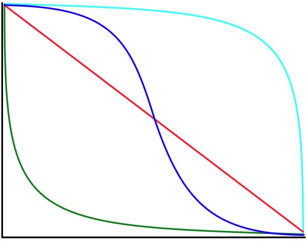
Decay Pattern

The decay classification portion of the pipeline buckets questions into a decay pattern based on how probability is distributed over time:

Constant Hazard

Some events could happen at any time with roughly equal probability. Earthquakes might fall into this classification. The chance of a major earthquake in Seattle next month is about the same whether we’re asking in January or December.

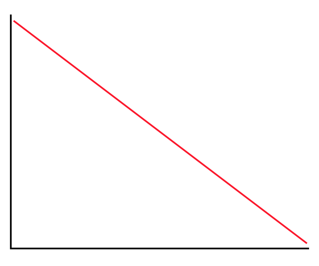
For constant hazard events, probability decays at a steady rate as time passes. Each month that passes without the event consumes a proportional slice of the cumulative probability. If 25% of your time window has elapsed without the event, you’ve consumed roughly 25% of the original probability.

Increasing Hazard

Some events have their probability concentrated near the deadline. The classic example is a debt ceiling negotiation. Neither side wants to blink early since maximum leverage comes from holding out. Maybe 10% of the probability is spread across the first eleven months, 35% is in the final two weeks excluding the last day, and 55% is on the last day before default.

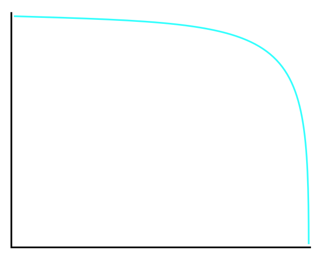
For increasing hazard events, probability decays very slowly at first. Early time passing without the event is expected—you’re not consuming much of the cumulative probability because there wasn’t much probability there to begin with. If eleven months pass without a deal, you’ve only burned through 10% of the total probability mass. As the deadline approaches and you enter the high-probability window, the decay rate accelerates.

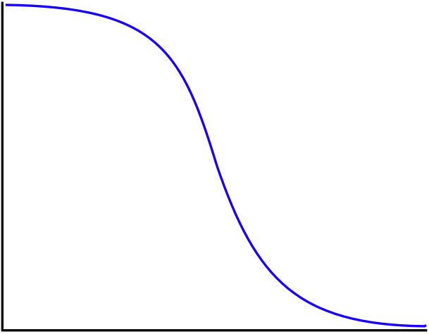
Decreasing Hazard

Some events have their probability concentrated early in the window. The classic example is a ceasefire. If it’s going to collapse, it’s most likely to collapse in the first few days or weeks. The probability of collapse is front-loaded.

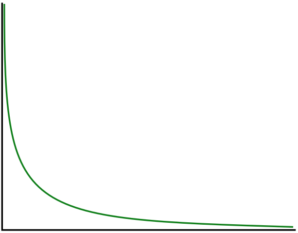
For decreasing hazard events, probability decays rapidly at first, then slows. Early survival is expensive. It burns through the front-loaded probability mass quickly. If a ceasefire holds for six months, most of the “collapse probability” has already been consumed without the event occurring. You’re now in the long tail where collapse was always unlikely, so further time passing costs you less.

Event-Driven Hazard

For completeness, I’ll mention another decay type that I use in forecasting, but didn’t implement due to complications. Sometimes, key events with a lot of probability mass happen at times that are not particularly close to either extreme.

An example might be a previously scheduled military exercise that could quickly pivot to an attack. If no attack materializes by the time the exercise is over and no further exercises are planned, it might be appropriate to expect the probability to decay rapidly afterward. As I mentioned, I did not implement this since it would be too easy for an AI to over-update on events.

How It Works

The decay analysis takes the method output and the hazard pattern, then calculates how much cumulative probability remains given how much time has elapsed.

Conceptually:

1. The method outputs a total probability P for the entire window

2. The hazard pattern defines how P is distributed across time

3. Given elapsed time t, we calculate how much of P has been “consumed” without the event occurring

4. The remaining probability is our updated estimate

For constant hazard, this is straightforward: linear decay. For increasing and decreasing hazard, the decay follows the shape of the probability distribution. Back-loaded distributions decay slowly then quickly; front-loaded distributions decay quickly then slowly.

Why It Matters

Decay functions matter most for questions with long time horizons where we’re partway through the window. If a question resolves in two weeks, there’s not much room for temporal dynamics to play out. If a question resolves in three years and we’re eighteen months in, the decay adjustment can meaningfully shift the estimate.

Consider a debt ceiling question at the start of the year with a December deadline. Your method might output 70% chance of a last-minute deal. In March, that 70% should barely have decayed as almost all the probability mass is still ahead of you. In November, it should still be close to 70%, because you’re just now entering the window where deals actually happen. Only if December arrives and passes without a deal does the probability finally collapse.

Contrast this with a ceasefire question. If your method outputs a 40% chance of collapse in the first year, and six months pass with the ceasefire holding, you’ve burned through most of that probability. Your updated estimate might be 10% or lower, not because new events have unfolded, but because the high-risk period has passed without incident.

Classification

How does the bot know which pattern applies? It’s part of the classification step. The LLM looks at the question structure and identifies cues:

• Negotiation dynamics → increasing hazard

• Random or memoryless processes → constant hazard

• Stability as evidence of equilibrium → decreasing hazard

Most questions default to constant hazard unless there’s clear structure suggesting otherwise. It’s the most conservative assumption. You’re not claiming to know something about temporal dynamics that you might be wrong about.

The Limits

Decay functions are a refinement, not a revolution. They adjust estimates at the margins based on temporal structure.

And the classification can be wrong. Some questions look like constant hazard but have hidden deadline pressure. Some look like decreasing hazard but have sleeper risks that compound over time. The decay function is only as good as the pattern recognition that assigns it.

As with everything in this pipeline, I’m tracking whether decay adjustments improve calibration.